The fractal snowflake, one of the most famous and mysterious geometric objects, was described by Helga von Koch at the beginning of our century. According to tradition, in our literature it is called Koch’s snowflake. This is a very “spiky” geometric figure, which can be metaphorically seen as the result of the Star of David being repeatedly “multiplied” by itself. Its six main rays are covered with an infinite number of large and small “needles” vertices. Every microscopic fragment of a snowflake’s contour is like two peas in a pod, and the large beam, in turn, contains an infinite number of the same microscopic fragments.

At an international symposium on the methodology of mathematical modeling in Varna back in 1994, I came across the work of Bulgarian authors who described their experience of using Koch’s snowflakes and other similar objects in high school lessons to illustrate the problem of the divisibility of space and the philosophical aporias of Zeno. In addition, from an educational point of view, in my opinion, the very principle of constructing regular fractal geometric structures is very interesting - the principle of recursive multiplication of the basic element. It’s not for nothing that nature “loves” fractal forms. This is explained precisely by the fact that they are obtained by simple reproduction and changing the size of a certain elementary building block. As you know, nature does not overflow with a variety of reasons and, where possible, makes do with the simplest algorithmic solutions. Look closely at the contours of the leaves, and in many cases you will find a clear relationship with the shape of the contour of a Koch snowflake.

Visualization of fractal geometric structures is possible only with the help of a computer. It is already very difficult to construct a Koch snowflake above the third order manually, but you really want to look into infinity! Therefore, why not try to develop an appropriate computer program. In RuNet you can find recommendations for building a Koch snowflake from triangles. The result of this algorithm looks like a jumble of intersecting lines. It is more interesting to combine this figure from “pieces”. The contour of a Koch snowflake consists of equal-length segments inclined at 0°, 60°, and 120° with respect to the horizontal x-axis. If we denote them 1, 2 and 3 respectively, then a snowflake of any order will consist of successive triplets - 1, 2, 3, 1, 2, 3, 1, 2, 3... etc. Each of these three types of segments can be attached to the previous one at one or the other end. Taking this circumstance into account, we can assume that the contour of a snowflake consists of segments of six types. Let's denote them 0, 1, 2, 3, 4, 5. Thus, we get the opportunity to encode a contour of any order using 6 digits (see figure).

A higher-order snowflake is obtained from a lower-order predecessor by replacing each edge with four, connected like folded palms (_/\_). Edge type 0 is replaced by four edges 0, 5, 1, 0 and so on according to the table:

0	0 1 5 0
1	1 2 0 1
2	2 3 1 2
3	3 4 2 3
4	4 5 3 4
5	5 0 4 5

A simple equilateral triangle can be thought of as a zero-order Koch snowflake. In the described encoding system, it corresponds to the entry 0, 4, 2. Everything else can be obtained by the described replacements. I will not provide the procedure code here and thereby deprive you of the pleasure of developing your own program. When writing it, it is not at all necessary to use an explicit recursive call. It can be replaced with a regular cycle. In the process of work, you will have another reason to think about recursion and its role in the formation of quasi-fractal forms of the world around us, and at the end of the path (if, of course, you are not too lazy to go through it to the end) you will be able to admire the complex pattern of the contours of a fractal snowflake, and also look finally in the face of infinity.

The geometric shape of the Koch snowflake looks like this



How to draw a Koch snowflake



And there is also the Koch pyramid



You can find out in more detail how to draw a Koch snowflake from the video below. Someone may understand, I gave up.

First, let's look at this Koch snowflake. The diagram below will best show us.



That is, to draw a given snowflake, you need to use individual geometric shapes, which make up this geometric fractal.



The basis of our drawing is an equilateral triangle. Each side is divided into three segments, from which the next, smaller, equilateral triangles are built. The same operation is performed with the resulting triangles several times.

Koch's snowflake is one of the first fractals studied by scientists. A snowflake is obtained from three copies of the Koch curve, information about this discovery appeared in 1904 in an article by the Swedish mathematician Helge von Koch. Essentially, a curve was invented as an example of a continuous line to which a tangent line cannot be drawn at any point. The Koch curve is simple in its design.

An example, a photo-drawing of a picture of a Koch snowflake with step-by-step drawing.



In this diagram you can examine in detail the lines that will later make a Koch snowflake.

And this is an interpretation of a new snowflake based on Koch’s snowflake.



Before you understand how to draw a Koch snowflake, we need to determine what it actually is.

So, a Koch snowflake is a geometric image - a fractal.

The full definition of Koch's snowflake is given in the picture below.

This figure is one of the first fractals studied by scientists. It is derived from three copies of the Koch curve, which first appeared in a paper by Swedish mathematician Helge von Koch in 1904. This curve was invented as an example of a continuous line that cannot be tangent to any point. Lines with this property were known before (Karl Weierstrass built his example back in 1872), but the Koch curve is remarkable for the simplicity of its design. It is no coincidence that his article is called “On a continuous curve without tangents, which arises from elementary geometry.”

How to build the Koch curve step by step.

The first iteration is simply the initial segment. Then it is divided into three equal parts, the central one is completed to form a regular triangle and then thrown out. The result is the second iteration - a broken line consisting of four segments. The same operation is applied to each of them, and the fourth step of construction is obtained. Continuing in the same spirit, you can get more and more new lines (all of them will be broken lines). And what happens in the limit (this will already be an imaginary object) is called the Koch curve.

Basic properties of the Koch curve

1.ABOUTis continuous, but nowhere differentiable. Roughly speaking, this is exactly why it was invented - as an example of this kind of mathematical “freaks”.

2. Has infinite length. Let the length of the original segment be equal to 1. At each construction step, we replace each of the segments that make up the line with a broken line, which 4/3 times longer. This means that the length of the entire broken line at each step is multiplied by 4/3 : the length of line number n is (4/3)n–1. Therefore, the limit line has no choice but to be infinitely long.

3.The Koch snowflake limits the finite area. And this despite the fact that its perimeter is infinite. This property may seem paradoxical, but it is obvious - a snowflake fits completely into a circle, so its area is obviously limited. The area can be calculated, and you don’t even need special knowledge for this - formulas for the area of ​​a triangle and the sum of a geometric progression are taught in school. For those interested, the calculation is listed below in fine print.

Let the side of the original regular triangle be equal to a. Then its area. First the side is 1 and the area is: . What happens as the iteration increases? We can assume that small equilateral triangles are attached to an existing polygon. The first time there are only 3 of them, and each next time there are 4 times more of them than the previous one. That is, at the nth step it will be completed Tn = 3 4n–1 triangles. The length of the side of each of them is one third of the side of the triangle completed in the previous step. This means it is equal to (1/3)n. Areas are proportional to the squares of the sides, so the area of ​​each triangle is . For large values ​​of n, this is, by the way, very small. The total contribution of these triangles to the area of ​​the snowflake is Tn Sn = 3/4 (4/9)n S0. Therefore, after the nth step, the area of ​​the figure will be equal to the sum S0 + T1 S1 + T2 S2 + ... +Tn Sn = . A snowflake is obtained after an infinite number of steps, which corresponds to n → ∞. The result is an infinite sum, but this is the sum of a decreasing geometric progression; there is a formula for it: . The area of ​​the snowflake is .

Options for constructing the Koch snowflake

The Koch snowflake “on the contrary” is obtained if we construct Koch curves inside the original equilateral triangle.

Cesaro lines. Instead of equilateral triangles, isosceles triangles with a base angle from 60° to 90° are used. In the figure, the angle is 88°.

Square option. Here the squares are completed.

This figure is one of the first fractals studied by scientists. It comes from three copies Koch curve, which first appeared in a paper by Swedish mathematician Helge von Koch in 1904. This curve was invented as an example of a continuous line that cannot be tangent to any point. Lines with this property were known before (Karl Weierstrass built his example back in 1872), but the Koch curve is remarkable for the simplicity of its design. It is no coincidence that his article is called “On a continuous curve without tangents, which arises from elementary geometry.”

Writing a function that calls itself recursively is one way to generate a fractal diagram on the screen. However, what if you wanted the rows in the above Cantor to be set as separate objects that could be moved independently? The recursive function is simple and elegant, but it doesn't allow you to do much beyond simply creating the template itself.

Here are the rules. The Koch curve and other fractal patterns are often called "mathematical monsters." This is due to the odd paradox that arises when you apply the recursive definition infinitely many times. If the length of the original starting line is one, the first iteration of the Koch curve will give a line length of four-thirds. Do it again and you get sixteen-nine. As you iterate into infinity, the length of the Koch curve approaches infinity. However, it fits into the tiny finite space provided right here on this paper!

The first stages of constructing the Koch curve

The drawing and animation perfectly show how the Koch curve is constructed step by step. The first iteration is simply the initial segment. Then it is divided into three equal parts, the central one is completed to form a regular triangle and then thrown out. The result is the second iteration - a broken line consisting of four segments. The same operation is applied to each of them, and the fourth step of construction is obtained. Continuing in the same spirit, you can get more and more new lines (all of them will be broken lines). And what happens in the limit (this will already be an imaginary object) is called the Koch curve.

Since we are working on the Earth of finite pixel processing, this theoretical paradox will not be a factor for us. We could proceed in the same way as with the Cantor set and write a recursive function that iteratively applies Koch's rules over and over again. However, we will solve this problem differently by treating each segment of the Koch curve as a separate object. This will open up some design possibilities. For example, if each segment is an object, we can allow each segment to move independently of its original location and participate in physics simulation.

Basic properties of the Koch curve

1. It is continuous, but nowhere differentiable. Roughly speaking, this is exactly why it was invented - as an example of this kind of mathematical “freaks”.

2. Has infinite length. Let the length of the original segment be equal to 1. At each construction step, we replace each of the segments that make up the line with a broken line, which is 4/3 times longer. This means that the length of the entire broken line is multiplied by 4/3 at each step: the length of the line with number n is equal to (4/3) n–1 . Therefore, the limit line has no choice but to be infinitely long.

Additionally, we could use random color, line thickness, etc. To display each segment differently. To accomplish our task of treating each segment as a separate object, we must first decide what the object should do. What features should it have?

Let's look at what we have. With the above elements, how and where do we apply Koch's rules and principles of recursion? In this simulation, we always followed two generations: the current one and the next one. When we finished calculating the next generation, it now became relevant and we moved on to calculating the new next generation.

3. Koch's snowflake limits the finite area. And this despite the fact that its perimeter is infinite. This property may seem paradoxical, but it is obvious - a snowflake fits completely into a circle, so its area is obviously limited. The area can be calculated, and you don’t even need special knowledge for this - formulas for the area of ​​a triangle and the sum of a geometric progression are taught in school. For those interested, the calculation is listed below in fine print.

We will use a similar technique here. This is what the code looks like. Of course, the above excludes the actual "work" here that defines these rules. How do we split one line segment into four as described by the rules? The construction of a fractal is based on the concept of infinity. Step 2: We will divide this segment into three equal parts and raise an equilateral triangle on the central part. Step 3: On the four new segments we will perform the step.

Intersect the tool between the two objects, click on the circle. The Koch snowflake is a special fractal curve constructed by the Koch mathematician, starting with Koch's lace. This is a curve drawn along the sides of an equilateral triangle. Koch laces are built on each side of the triangle.

Let the side of the original regular triangle be equal to a. Then its area. First the side is 1 and the area is: . What happens as the iteration increases? We can assume that small equilateral triangles are attached to an existing polygon. The first time there are only 3 of them, and each next time there are 4 times more of them than the previous one. That is, on n At the th step, T n = 3 · 4 n–1 triangles will be completed. The length of the side of each of them is one third of the side of the triangle completed in the previous step. This means it is equal to (1/3) n. Areas are proportional to the squares of the sides, so the area of ​​each triangle is . For large values n By the way, this is very little. The total contribution of these triangles to the area of ​​the snowflake is T n · S n = 3/4 · (4/9) n · S 0 . Therefore after n th step, the area of ​​the figure will be equal to the sum S 0 + T 1 · S 1 + T 2 · S 2 + ... +T n · S n = . A snowflake is obtained after an infinite number of steps, which corresponds to n → ∞. The result is an infinite sum, but this is the sum of a decreasing geometric progression; there is a formula for it: . The area of ​​the snowflake is equal.

The following table shows the first steps in constructing a curve. To create a fractal, you simply need to insert three copies of the curve along the sides of the triangle. Note that the second figure is the Star of David. The end result is a closed curve built on an equilateral triangle. It may be noted that the frit contains a six-pointed star. The design is very similar to a fractal pentagonal one.

There is another way to build snowflakes. The construction described above can be defined as a construction by addition, since the starting figure, the triangle, adds other elements. There is a substructure that removes elements instead of the original shape.

4. The fractal dimension is log4/log3 = log 3 4 ≈ 1.261859... . Accurate calculation will require considerable effort and detailed explanations, so here is rather an illustration of the definition of fractal dimension. From the power law formula N(δ) ~ (1/δ)D, where N- number of intersecting squares, δ - their size, D- dimension, we obtain that D = log 1/δ N. This equality is true up to the addition of a constant (the same for all δ ). The figures show the fifth iteration of constructing the Koch curve; the grid squares that intersect with it are shaded green. The length of the original segment is 1, so in the left figure the side length of the squares is 1/9. 12 squares are shaded, log 9 12 ≈ 1.130929... . Not very similar to 1.261859 yet... . Let's look further. In the middle picture, the squares are half the size, their size is 1/18, shaded 30. log 18 30 ≈ 1.176733... . Already better. On the right, the squares are still half as large, 72 pieces have already been painted over. log 72 30 ≈ 1.193426... . Even closer. Then you need to increase the iteration number and at the same time decrease the squares, then the “empirical” value of the dimension of the Koch curve will steadily approach log 3 4, and in the limit it will completely coincide.

Options

Koch's snowflake "in reverse" obtained if we construct Koch curves inside the original equilateral triangle.

Cesaro Lines. Instead of equilateral triangles, isosceles triangles with a base angle from 60° to 90° are used. In the figure, the angle is 88°.

Square option. Here the squares are completed.

Three-dimensional analogues. Koch space.

It was an unusually warm winter in Boston, but we still waited for the first snowfall. Watching the snow fall through the window, I thought about snowflakes and how their structure is not at all easy to describe mathematically. There is however one special kind of snowflake, known as the Koch snowflake, which can be described relatively simply. Today we'll look at how its shape can be built using the COMSOL Multiphysics Application Builder.

The Making of Koch's Snowflake

As we already mentioned in our blog, fractals can be used in . Snowflake Koch is a fractal, which is notable in that there is a very simple iterative process to construct it:

1. Let's start with an equilateral triangle, which is actually the zeroth iteration of the Koch snowflake.
2. Let's find the center point on each edge of the current snowflake.
3. In the center of each edge, add an equilateral triangle protruding outwards with a side equal to 1/3 of the length of the current edge.
4. Let's define the next iteration of the Koch snowflake to be on the outside of the previous snowflake and all the added triangles.
5. Repeat steps 2-4 as many times as necessary.

This procedure is illustrated in the figure below for the first four iterations of drawing a snowflake.

The first four iterations of the Koch snowflake. Image by Wxs - Own work. Licensed under CC BY-SA 3.0, via Wikimedia Commons.

Construction of the Koch snowflake geometry

Since we now know which algorithm to use, let's look at how to create such a structure using the COMSOL Multiphysics Application Builder. We'll open a new file and create a 2D object geometry part at the node Global definitions. For this object, we will set five input parameters: the length of the side of an equilateral triangle; X- And y– coordinates of the midpoint of the base; and components of the normal vector directed from the middle of the base to the opposite vertex, as shown in the figures below.

Five parameters used to set the size, position, and orientation of an equilateral triangle.

Setting the input parameters of the geometric part.
A polygon primitive is used to construct an equilateral triangle.

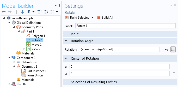
The object can rotate around the center of the bottom edge.

An object can be moved relative to the origin.

Now that we have defined the geometric part, we use it once in the section Geometry. This single triangle is equivalent to the zeroth iteration of the Koch snowflake, and now let's use the Application Builder to create more complex snowflakes.

App UI Markup in the Application Builder

The application has a very simple user interface. It contains only two components that the user can interact with: Slider (Slider)(marked as 1 in the figure below), with which you can set the number of iterations needed to create a snowflake, and Button(label 2), by clicking which the resulting geometry is created and displayed. There are also Text inscription(label 3) and Display (Display) of data(label 4), which show the number of specified iterations, as well as the window Charts(label 5), which displays the final geometry.

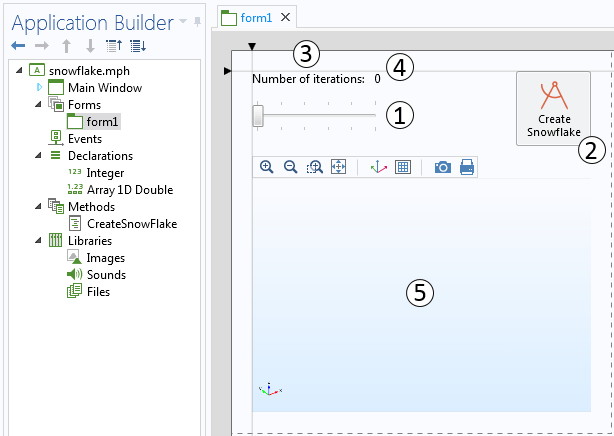
The application has one single form with five components.

The application has two Definitions, one of which defines an integer value called Iterations, which defaults to zero but can be changed by the user. A 1D array of doubles called Center is also defined. The single element in the array has a value of 0.5, which is used to find the center point of each edge. This value never changes.

Settings for two Definitions.

The Slider component in the UI controls the value of the integer, Iterations parameter. The screenshot below shows the settings for the "Slider" and the values, which are set as integers in the range between 0 and 5. The same source (as for the slider) is also selected for the component Data Display to display the number of specified iterations on the application screen. We limit the potential user to five iterations because the algorithm used is suboptimal and not very efficient, but is simple enough to implement and demonstrate.

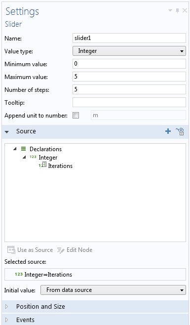
Settings for the "Slider" component.

Next, let's look at the settings for our button, shown in the screenshot below. When the button is pressed, two commands are executed. First, the CreateSnowFlake method is called. The resulting geometry is then displayed in the graphics window.

Button settings.

We have now looked at the user interface of our application and we can see that the creation of any snowflake geometry must happen through a method called. Let's look at the code for this method, with line numbering added to the left and string constants highlighted in red:

1 model.geom("geom1" ).feature().clear(); 2 model.geom("geom1" ).create("pi1" , "PartInstance" ); 3 model.geom("geom1" ).run("fin" ); 4 for (int iter = 1; iter "geom1" ).getNEdges()+1; 6 UnionList = "pi" + iter; 7 for (int edge = 1; edge "geom1" ).getNEdges(); edge++) ( 8 String newPartInstance = "pi" + iter + edge; 9 model.geom("geom1" ).create(newPartInstance, "PartInstance" ).set("part" , "part1" ); 10 with(model. geom("geom1" ).feature(newPartInstance)); 11 setEntry("inputexpr" , "Length" , toString(Math.pow(1.0/3.0, iter))); 12 setEntry("inputexpr" , "px" , model.geom("geom1" ).edgeX(edge, Center)); 13 setEntry("inputexpr" , "py" , model.geom("geom1" ).edgeX(edge, Center)); 14 setEntry("inputexpr " , "nx" , model.geom("geom1" ).edgeNormal(edge, Center)); 15 setEntry("inputexpr" , "ny" , model.geom("geom1" ).edgeNormal(edge, Center)) ; 16 endwith(); 17 UnionList = newPartInstance; 18 ) 19 model.geom("geom1" ).create("pi" +(iter+1), "Union" ).selection("input" ).set(UnionList ); 20 model.geom("geom1" ).feature("pi" +(iter+1)).set("intbnd" , "off" ); 21 model.geom("geom1" ).run("fin" ); 22)

Let's go through the code line by line to understand what function each line performs:

1. Clearing all existing geometric sequences so we can start from scratch.
2. We create one instance of the object - our "triangle", using the default size, orientation and location. This is our zeroth order snowflake with identifier label pi1.
3. Let's finalize the geometry. This operation is required to update all geometry indexes.
4. Let's begin the process of iterating through all given iterations of the snowflake, using the Iterations definition as a stopping condition.
5. We define an empty array of strings, UnionList. Each element of the array contains an identifier of various geometric objects. The length of this array is equal to the number of edges in the last iteration plus one.
6. We define the first element in the UnionList array. It is an identifier of the result of the previous iteration. Keep in mind that iteration zero has already been created in lines 1-3. The integer value iter is automatically converted to a string and appended to the end of the string "pi" .
7. We go through the number of edges in the previously generated snowflake.
8. We set an identifier label for a new instance of an object accessing from the “triangle” part instance that is created on this edge. Note that the integer values ​​iter and edge are sequentially added to the end of the string pi , the object instance's identifier label.
9. We create an instance of the "triangle" object and assign it the identifier label that was just specified.
10. We indicate that lines 11-15 refer to the current instance of the object (part instance) using the with()/endwith() statement.
11. Determine the length of the side of the triangle. The zeroth order has a side length of one, so the nth iteration has a side length of (1/3)n. The toString() function is required to cast (convert) data types - a floating point number to a string.
12. We set x-coordinate of the new triangle, as the center point of the side of the last iteration. The edgeX method is documented in . Recall that Center is set to 0.5.
13. We set y-coordinate.
14. We set x-component of the normal vector of the triangle. The edgeNormal method is also documented in COMSOL Programming Reference Manual.
15. We set y-component of the normal vector.
16. We close the with()/endwith() statement.
17. Add a label-identifier of the current triangle to the list of all objects.
18. We close the search of all edges.
19. We create a Boolean Union (logical union) of all objects into a geometric sequence. We assign a new value pi to the label N, where N is the number next iterations. Parentheses are required around (iter+1) so that the incremented iter value is converted to a string.
20. We indicate that the internal boundaries of the final object are not preserved.
21. Let's finalize the geometry. The last operation updates all geometry indexes for the next iteration of the snowflake.
22. We close the cycle of iterations of creating a snowflake.

Thus, we have covered all aspects and elements of our application. Let's look at the results!

Our simple application for constructing the Koch snowflake.

We could extend our application to write geometry to a file, or even perform additional analyzes directly. For example, we could design a fractal antenna. If you are interested in the design of the antenna, check out our example, or even make its layout from scratch.

Try it yourself

If you want to build this application yourself, but have not yet completed the Application Builder, you may find the following resources helpful:

• Download the guide Introduction to the Application Development Environment in English
• Watch these videos and learn how to use
• Read these topics to become familiar with how simulation applications are used in

Once you've covered this material, you'll see how the app's functionality can be expanded to resize a snowflake, export created geometry, estimate area and perimeter, and much more.

What kind of application would you like to create in COMSOL Multiphysics? for help.

Similar articles